Seurat单细胞处理流程之三:降维&注释
rm(list = ls())
setwd("/mnt/DEV_8T/zhaozm/seurat全流程/降维注释")
## 设置保存的目录
## 数据目录
data_dir <- "/mnt/DEV_8T/zhaozm/seurat全流程/降维注释/data"
if (!dir.exists(data_dir)) {
  dir.create(data_dir, recursive = TRUE)
}
## 图片目录
img_dir <- "/mnt/DEV_8T/zhaozm/seurat全流程/降维注释/img"

if (!dir.exists(img_dir)) {
  dir.create(img_dir, recursive = TRUE)
}
library(Seurat)
library(dplyr)
library(readr)
library(Matrix)
library(ggplot2)
library(patchwork)
library(tidyverse)
library(tidydr)
library(RColorBrewer)
library(scales)
library(ggpubr)
library(ggplotify)
library(pheatmap)
library(reshape2)
library(gplots)
set.seed(123)
载入需要的程序包:SeuratObject
载入需要的程序包:sp
载入程序包:‘SeuratObject’
The following objects are masked from ‘package:base’:
intersect, t
载入程序包:‘dplyr’
The following objects are masked from ‘package:stats’:
filter, lag
The following objects are masked from ‘package:base’:
intersect, setdiff, setequal, union
── [1mAttaching core tidyverse packages[22m ──────────────────────── tidyverse 2.0.0 ──
[32m✔[39m [34mforcats [39m 1.0.0 [32m✔[39m [34mstringr [39m 1.5.1
[32m✔[39m [34mlubridate[39m 1.9.4 [32m✔[39m [34mtibble [39m 3.2.1
[32m✔[39m [34mpurrr [39m 1.0.2 [32m✔[39m [34mtidyr [39m 1.3.1
── [1mConflicts[22m ────────────────────────────────────────── tidyverse_conflicts() ──
[31m✖[39m [34mtidyr[39m::[32mexpand()[39m masks [34mMatrix[39m::expand()
[31m✖[39m [34mdplyr[39m::[32mfilter()[39m masks [34mstats[39m::filter()
[31m✖[39m [34mdplyr[39m::[32mlag()[39m masks [34mstats[39m::lag()
[31m✖[39m [34mtidyr[39m::[32mpack()[39m masks [34mMatrix[39m::pack()
[31m✖[39m [34mtidyr[39m::[32munpack()[39m masks [34mMatrix[39m::unpack()
[36mℹ[39m Use the conflicted package ([3m[34m<http://conflicted.r-lib.org/>[39m[23m) to force all conflicts to become errors
载入程序包:‘scales’
The following object is masked from ‘package:purrr’:
discard
The following object is masked from ‘package:readr’:
col_factor
载入程序包:‘reshape2’
The following object is masked from ‘package:tidyr’:
smiths
载入程序包:‘gplots’
The following object is masked from ‘package:stats’:
lowess
# 读取上一步的rds文件
pbmc <- read_rds(file = "../数据质控/pbmc_f.rds")
#将表达数据标准化
pbmc <- NormalizeData(pbmc, normalization.method = "LogNormalize", scale.factor = 10000)
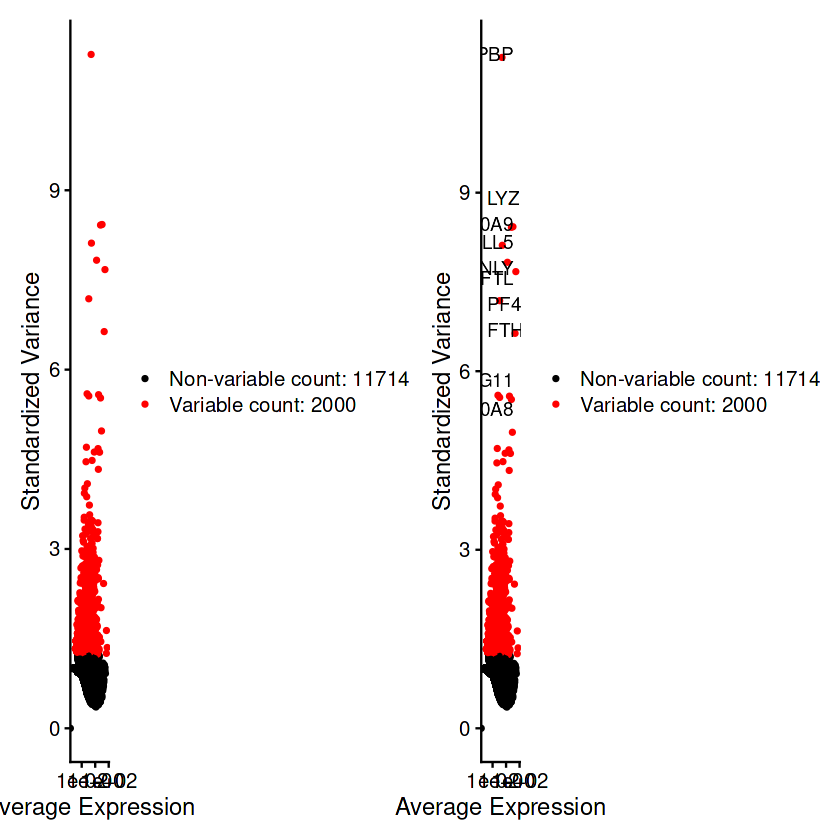
#寻找高变基因
pbmc <- FindVariableFeatures(pbmc, selection.method = "vst", nfeatures = 2000)
top10 <- head(VariableFeatures(pbmc), 10)#查看十个程度最强的高变基因
plot1 <- VariableFeaturePlot(pbmc)
plot2 <- LabelPoints(plot = plot1, points = top10, repel = TRUE)
plot1 + plot2
Normalizing layer: counts
Finding variable features for layer counts
When using repel, set xnudge and ynudge to 0 for optimal results
Warning message in scale_x_log10():
“[1m[22m[32mlog-10[39m transformation introduced infinite values.”
Warning message in scale_x_log10():
“[1m[22m[32mlog-10[39m transformation introduced infinite values.”
#scale全部基因
pbmc <- ScaleData(pbmc, features = rownames(pbmc))
Centering and scaling data matrix
## 执行PCA降维
pbmc <- RunPCA(pbmc, features = VariableFeatures(object = pbmc))
## 保存
write_rds(x = pbmc,file = "./data/pbmc_pca.rds")
PC_ 1
Positive:  CST3, TYROBP, LST1, AIF1, FTL, FTH1, LYZ, FCN1, S100A9, TYMP
	   FCER1G, CFD, LGALS1, S100A8, CTSS, LGALS2, SERPINA1, IFITM3, SPI1, CFP
	   PSAP, IFI30, SAT1, COTL1, S100A11, NPC2, GRN, LGALS3, GSTP1, PYCARD
Negative:  MALAT1, LTB, IL32, IL7R, CD2, B2M, ACAP1, CD27, STK17A, CTSW
	   CD247, GIMAP5, AQP3, CCL5, SELL, TRAF3IP3, GZMA, MAL, CST7, ITM2A
	   MYC, GIMAP7, HOPX, BEX2, LDLRAP1, GZMK, ETS1, ZAP70, TNFAIP8, RIC3
PC_ 2
Positive:  CD79A, MS4A1, TCL1A, HLA-DQA1, HLA-DQB1, HLA-DRA, LINC00926, CD79B, HLA-DRB1, CD74
	   HLA-DMA, HLA-DPB1, HLA-DQA2, CD37, HLA-DRB5, HLA-DMB, HLA-DPA1, FCRLA, HVCN1, LTB
	   BLNK, P2RX5, IGLL5, IRF8, SWAP70, ARHGAP24, FCGR2B, SMIM14, PPP1R14A, C16orf74
Negative:  NKG7, PRF1, CST7, GZMB, GZMA, FGFBP2, CTSW, GNLY, B2M, SPON2
	   CCL4, GZMH, FCGR3A, CCL5, CD247, XCL2, CLIC3, AKR1C3, SRGN, HOPX
	   TTC38, APMAP, CTSC, S100A4, IGFBP7, ANXA1, ID2, IL32, XCL1, RHOC
PC_ 3
Positive:  HLA-DQA1, CD79A, CD79B, HLA-DQB1, HLA-DPB1, HLA-DPA1, CD74, MS4A1, HLA-DRB1, HLA-DRA
	   HLA-DRB5, HLA-DQA2, TCL1A, LINC00926, HLA-DMB, HLA-DMA, CD37, HVCN1, FCRLA, IRF8
	   PLAC8, BLNK, MALAT1, SMIM14, PLD4, P2RX5, IGLL5, LAT2, SWAP70, FCGR2B
Negative:  PPBP, PF4, SDPR, SPARC, GNG11, NRGN, GP9, RGS18, TUBB1, CLU
	   HIST1H2AC, AP001189.4, ITGA2B, CD9, TMEM40, PTCRA, CA2, ACRBP, MMD, TREML1
	   NGFRAP1, F13A1, SEPT5, RUFY1, TSC22D1, MPP1, CMTM5, RP11-367G6.3, MYL9, GP1BA
PC_ 4
Positive:  HLA-DQA1, CD79B, CD79A, MS4A1, HLA-DQB1, CD74, HIST1H2AC, HLA-DPB1, PF4, SDPR
	   TCL1A, HLA-DRB1, HLA-DPA1, HLA-DQA2, PPBP, HLA-DRA, LINC00926, GNG11, SPARC, HLA-DRB5
	   GP9, AP001189.4, CA2, PTCRA, CD9, NRGN, RGS18, CLU, TUBB1, GZMB
Negative:  VIM, IL7R, S100A6, IL32, S100A8, S100A4, GIMAP7, S100A10, S100A9, MAL
	   AQP3, CD2, CD14, FYB, LGALS2, GIMAP4, ANXA1, CD27, FCN1, RBP7
	   LYZ, S100A11, GIMAP5, MS4A6A, S100A12, FOLR3, TRABD2A, AIF1, IL8, IFI6
PC_ 5
Positive:  GZMB, NKG7, S100A8, FGFBP2, GNLY, CCL4, CST7, PRF1, GZMA, SPON2
	   GZMH, S100A9, LGALS2, CCL3, CTSW, XCL2, CD14, CLIC3, S100A12, RBP7
	   CCL5, MS4A6A, GSTP1, FOLR3, IGFBP7, TYROBP, TTC38, AKR1C3, XCL1, HOPX
Negative:  LTB, IL7R, CKB, VIM, MS4A7, AQP3, CYTIP, RP11-290F20.3, SIGLEC10, HMOX1
	   LILRB2, PTGES3, MAL, CD27, HN1, CD2, GDI2, CORO1B, ANXA5, TUBA1B
	   FAM110A, ATP1A1, TRADD, PPA1, CCDC109B, ABRACL, CTD-2006K23.1, WARS, VMO1, FYB
# 定义数据集的“维度”
#NOTE: This process can take a long time for big datasets, comment out for expediency.
#More approximate techniques such as those implemented in ElbowPlot() can be used to reduce computation time
pbmc <- JackStraw(pbmc, num.replicate = 100,dims = 30)
pbmc <- ScoreJackStraw(pbmc, dims = 1:30)
pdf("./img/elbow_score.pdf",width = 12,height = 8)
JackStrawPlot(pbmc, dims = 1:30)
dev.off()

## JackStraw函数运行时间特别久
Warning message:
“[1m[22mRemoved 50411 rows containing missing values or values outside the scale range
(`geom_point()`).”
pdf: 2
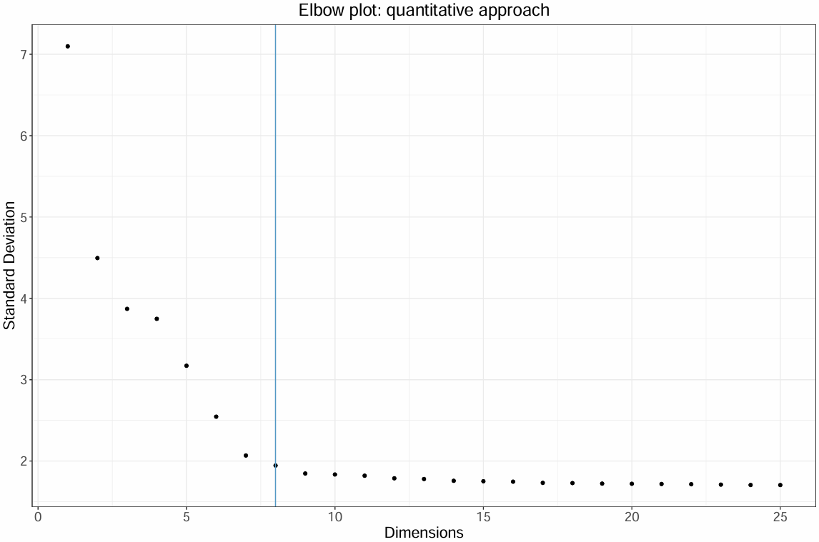
#通过筛选贡献小于5%方差和累计贡献90%方差的PC截断点作为曲线拐点
#连续PC之间的差异方差贡献百分比变化小于0.1%的点作为曲线拐点
pct <-pbmc[["pca"]]@stdev /sum(pbmc[["pca"]]@stdev) * 100
cumu <- cumsum(pct)

#选择
pc.use <-min(which(cumu >90&pct < 5)[1],
             sort(which((pct[1:length(pct) - 1] - pct[2:length(pct)])>0.1),decreasing = T)[1]+1)
# 保存为 PDF 文件
pdf("./img/elbow_score2.pdf", width = 12, height = 8)


# 绘制 Elbow Plot 并调整字体大小
ElbowPlot(pbmc, ndims = 25)$data %>%
  ggplot() +
  geom_point(aes(x = dims, y = stdev)) +
  geom_vline(xintercept = pc.use, color = "#5399C4") +
  theme_bw() +
  labs(
    title = "Elbow plot: quantitative approach",
    x = "Dimensions",
    y = "Standard Deviation"
  ) +
  theme(
    plot.title = element_text(size = 18, hjust = 0.5),  # 标题字体大小并居中
    axis.title.x = element_text(size = 16),  # X轴标题字体大小
    axis.title.y = element_text(size = 16),  # Y轴标题字体大小
    axis.text.x = element_text(size = 14),   # X轴刻度字体大小
    axis.text.y = element_text(size = 14)    # Y轴刻度字体大小
  )

# 关闭 PDF 文件
dev.off()


#可以看每个pc的方差
Stdev(pbmc)
## 保存这一步的文件
write_rds(pbmc,file = "./data/dim_res_pbmc.rds")
结果如下:
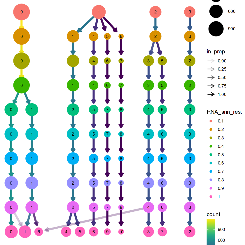
####调试resolution####
# a、尝试不同分辨率下的细胞分群
library(clustree)
set.seed(123)

pbmc <- FindNeighbors(pbmc, reduction = "pca", dims = 1:15)
pbmc <- FindClusters(
  object = pbmc,
  resolution = c( seq( 0.1, 1, 0.1) ) # 分辨率从 0.1,-1,间隔 0.1 一档
)


# 可视化
clustree(pbmc@meta.data, prefix = "RNA_snn_res.")
## 确定为0.5较为合理
载入需要的程序包:ggraph


载入程序包:‘ggraph’


The following object is masked from ‘package:sp’:

    geometry


Computing nearest neighbor graph

Computing SNN


Modularity Optimizer version 1.3.0 by Ludo Waltman and Nees Jan van Eck

Number of nodes: 2638
Number of edges: 106339

Running Louvain algorithm...
Maximum modularity in 10 random starts: 0.9615
Number of communities: 4
Elapsed time: 0 seconds
Modularity Optimizer version 1.3.0 by Ludo Waltman and Nees Jan van Eck

Number of nodes: 2638
Number of edges: 106339

Running Louvain algorithm...
Maximum modularity in 10 random starts: 0.9338
Number of communities: 7
Elapsed time: 0 seconds
Modularity Optimizer version 1.3.0 by Ludo Waltman and Nees Jan van Eck

Number of nodes: 2638
Number of edges: 106339

Running Louvain algorithm...
Maximum modularity in 10 random starts: 0.9097
Number of communities: 8
Elapsed time: 0 seconds
Modularity Optimizer version 1.3.0 by Ludo Waltman and Nees Jan van Eck

Number of nodes: 2638
Number of edges: 106339

Running Louvain algorithm...
Maximum modularity in 10 random starts: 0.8871
Number of communities: 8
Elapsed time: 0 seconds
Modularity Optimizer version 1.3.0 by Ludo Waltman and Nees Jan van Eck

Number of nodes: 2638
Number of edges: 106339

Running Louvain algorithm...
Maximum modularity in 10 random starts: 0.8680
Number of communities: 9
Elapsed time: 0 seconds
Modularity Optimizer version 1.3.0 by Ludo Waltman and Nees Jan van Eck

Number of nodes: 2638
Number of edges: 106339

Running Louvain algorithm...
Maximum modularity in 10 random starts: 0.8525
Number of communities: 9
Elapsed time: 0 seconds
Modularity Optimizer version 1.3.0 by Ludo Waltman and Nees Jan van Eck

Number of nodes: 2638
Number of edges: 106339

Running Louvain algorithm...
Maximum modularity in 10 random starts: 0.8370
Number of communities: 9
Elapsed time: 0 seconds
Modularity Optimizer version 1.3.0 by Ludo Waltman and Nees Jan van Eck

Number of nodes: 2638
Number of edges: 106339

Running Louvain algorithm...
Maximum modularity in 10 random starts: 0.8215
Number of communities: 9
Elapsed time: 0 seconds
Modularity Optimizer version 1.3.0 by Ludo Waltman and Nees Jan van Eck

Number of nodes: 2638
Number of edges: 106339

Running Louvain algorithm...
Maximum modularity in 10 random starts: 0.8059
Number of communities: 9
Elapsed time: 0 seconds
Modularity Optimizer version 1.3.0 by Ludo Waltman and Nees Jan van Eck

Number of nodes: 2638
Number of edges: 106339

Running Louvain algorithm...
Maximum modularity in 10 random starts: 0.7932
Number of communities: 11
Elapsed time: 0 seconds
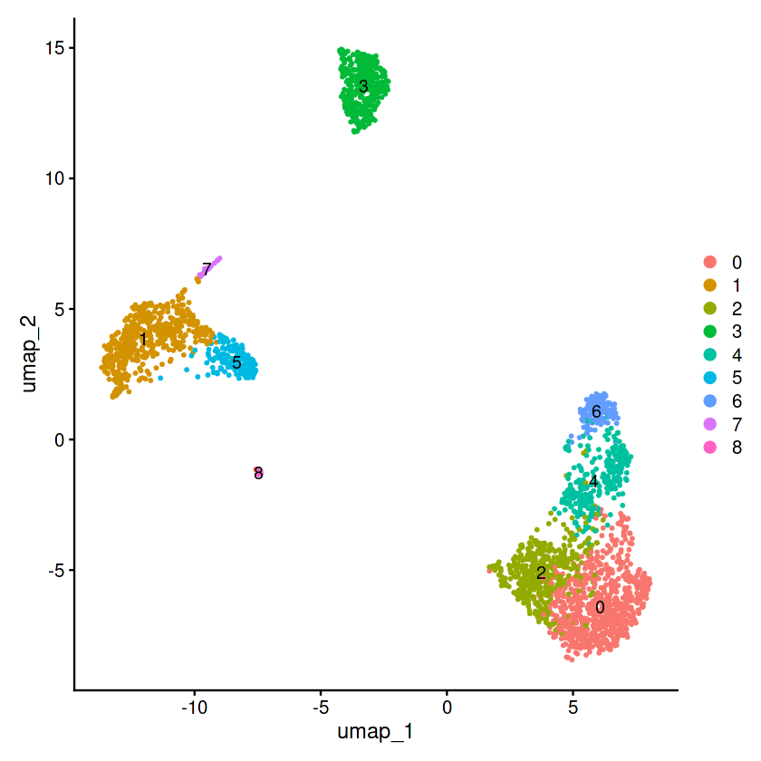
## 按照最佳的维度和分辨率进行筛选
## 读取之前pca的结果
pbmc <- read_rds(file.path(data_dir,  "pbmc_pca.rds"))
pbmc <- FindNeighbors(pbmc, dims = 1:8)
pbmc <- FindClusters(pbmc, resolution = 0.5)

# umap可视化
pbmc <- RunUMAP(pbmc, dims = 1:15)
p=DimPlot(pbmc, reduction = "umap",label = T)
p
Computing nearest neighbor graph

Computing SNN


Modularity Optimizer version 1.3.0 by Ludo Waltman and Nees Jan van Eck

Number of nodes: 2638
Number of edges: 91842

Running Louvain algorithm...
Maximum modularity in 10 random starts: 0.8813
Number of communities: 9
Elapsed time: 0 seconds


Warning message:
“The default method for RunUMAP has changed from calling Python UMAP via reticulate to the R-native UWOT using the cosine metric
To use Python UMAP via reticulate, set umap.method to 'umap-learn' and metric to 'correlation'
This message will be shown once per session”
15:40:34 UMAP embedding parameters a = 0.9922 b = 1.112

15:40:34 Read 2638 rows and found 15 numeric columns

15:40:34 Using Annoy for neighbor search, n_neighbors = 30

15:40:34 Building Annoy index with metric = cosine, n_trees = 50

0%   10   20   30   40   50   60   70   80   90   100%

[----|----|----|----|----|----|----|----|----|----|

*
*
*
*
*
*
*
*
*
*
*
*
*
*
*
*
*
*
*
*
*
*
*
*
*
*
*
*
*
*
*
*
*
*
*
*
*
*
*
*
*
*
*
*
*
*
*
*
*
*
|

15:40:34 Writing NN index file to temp file /tmp/RtmpzRaEd4/file4242620826088

15:40:34 Searching Annoy index using 1 thread, search_k = 3000

15:40:35 Annoy recall = 100%

15:40:35 Commencing smooth kNN distance calibration using 1 thread
 with target n_neighbors = 30

15:40:36 Initializing from normalized Laplacian + noise (using RSpectra)

15:40:36 Commencing optimization for 500 epochs, with 107666 positive edges

15:40:39 Optimization finished
# 寻找marker基因并对cluster进行重命名
pbmc.markers <- FindAllMarkers(pbmc, only.pos = TRUE,
                               min.pct = 0.25, logfc.threshold = 0.25)
pbmc.markers %>% group_by(cluster) %>% top_n(n = 2, wt = avg_log2FC)

# top5 <- pbmc.markers %>% group_by(cluster) %>% top_n(n = 5, wt = avg_log2FC)
top10 <- pbmc.markers %>% group_by(cluster) %>% top_n(n = 10, wt = avg_log2FC)
# top20 <- pbmc.markers %>% group_by(cluster) %>% top_n(n = 20, wt = avg_log2FC)
# top50 <- pbmc.markers %>% group_by(cluster) %>% top_n(n = 50, wt = avg_log2FC)
# write.csv(top50, file.path(data_dir, "cellmarkertop50.csv"), row.names = FALSE)
# write.csv(top20, file.path(data_dir, "cellmarkertop20.csv"), row.names = FALSE)
write.csv(top10, file.path(data_dir, "cellmarkertop10.csv"), row.names = FALSE)
Calculating cluster 0

Calculating cluster 1

Calculating cluster 2

Calculating cluster 3

Calculating cluster 4

Calculating cluster 5

Calculating cluster 6

Calculating cluster 7

Calculating cluster 8
| p_val | avg_log2FC | pct.1 | pct.2 | p_val_adj | cluster | gene |
|---|---|---|---|---|---|---|
| <dbl> | <dbl> | <dbl> | <dbl> | <dbl> | <fct> | <chr> |
| 3.518916e-81 | 2.381647 | 0.429 | 0.109 | 4.825841e-77 | 0 | CCR7 |
| 8.349070e-50 | 2.110239 | 0.333 | 0.102 | 1.144991e-45 | 0 | LEF1 |
| 3.643533e-138 | 7.273517 | 0.298 | 0.004 | 4.996741e-134 | 1 | FOLR3 |
| 1.448440e-120 | 6.730405 | 0.275 | 0.006 | 1.986390e-116 | 1 | S100A12 |
| 3.535948e-57 | 2.102440 | 0.423 | 0.113 | 4.849199e-53 | 2 | AQP3 |
| 1.572168e-38 | 1.988128 | 0.277 | 0.068 | 2.156071e-34 | 2 | CD40LG |
| 2.397625e-272 | 7.379757 | 0.564 | 0.009 | 3.288103e-268 | 3 | LINC00926 |
| 2.745016e-237 | 7.135051 | 0.488 | 0.007 | 3.764515e-233 | 3 | VPREB3 |
| 1.200580e-167 | 4.436781 | 0.591 | 0.056 | 1.646476e-163 | 4 | GZMK |
| 1.895709e-90 | 3.570035 | 0.431 | 0.061 | 2.599775e-86 | 4 | GZMH |
| 6.034160e-214 | 5.438328 | 0.509 | 0.010 | 8.275247e-210 | 5 | CDKN1C |
| 6.153970e-169 | 5.890728 | 0.373 | 0.005 | 8.439554e-165 | 5 | CKB |
| 1.830897e-267 | 6.011786 | 0.986 | 0.070 | 2.510892e-263 | 6 | GZMB |
| 1.867633e-181 | 6.197212 | 0.490 | 0.014 | 2.561272e-177 | 6 | AKR1C3 |
| 1.476034e-221 | 8.120790 | 0.533 | 0.002 | 2.024232e-217 | 7 | SERPINF1 |
| 1.010540e-200 | 7.600520 | 0.800 | 0.012 | 1.385855e-196 | 7 | FCER1A |
| 0.000000e+00 | 14.251143 | 0.571 | 0.000 | 0.000000e+00 | 8 | LY6G6F |
| 4.359585e-206 | 13.818529 | 0.357 | 0.000 | 5.978735e-202 | 8 | RP11-879F14.2 |
# 保存这一步的pbmc数据
write_rds(pbmc, file = file.path(data_dir, "pbmcumap.rds"))
## 通过网站确定pbmc的注释结果
# 读取上一步的rds文件
pbmc <- read_rds(file.path(data_dir, "pbmcumap.rds"))
unique(pbmc$RNA_snn_res.0.5)
p=DimPlot(pbmc, reduction = "umap",label = T)
p

# 进一步细胞注释
celltype=data.frame(ClusterID=0:16,
                    celltype='unkown')
celltype[celltype$ClusterID %in% c(0),2]='Naive CD4 T'
celltype[celltype$ClusterID %in% c(1),2]='CD14+ Mono'
celltype[celltype$ClusterID %in% c(2),2]='Memory CD4 T'
celltype[celltype$ClusterID %in% c(3),2]='B'
celltype[celltype$ClusterID %in% c(4),2]='CD8 T'
celltype[celltype$ClusterID %in% c(5),2]='FCGR3A+ Mono'
celltype[celltype$ClusterID %in% c(6),2]='NK'
celltype[celltype$ClusterID %in% c(7),2]='DC'
celltype[celltype$ClusterID %in% c(8),2]='Platelet'


celltype
table(celltype$celltype)

#先加一列celltype所有值为空
pbmc@meta.data$celltype = "NA"
###注释
for(i in 1:nrow(celltype)){
  pbmc@meta.data[which(pbmc@meta.data$seurat_clusters == celltype$ClusterID[i]),'celltype'] <- celltype$celltype[i]}

table(pbmc@meta.data$celltype)

Idents(pbmc) <- "seurat_clusters"
Idents(pbmc) <- "celltype"

## 查看dim图
p = DimPlot(pbmc, reduction = "umap",label = T)
p
DimPlot(pbmc, reduction = "umap",label = T,split.by = "group")
## 保存注释之后的文件
write_rds(pbmc ,file = "./data/pbmc注释后.rds")