Seurat单细胞处理流程之四：差异分析&富集分析

25 Mar 2025

简介

整体来说，单细胞的差异分析与普通转录组的差异分析流程类似，但是原理略有不同。（补充几个常用包的原理和秩和检验的原理）

1.差异分析

rm(list = ls())
setwd("/mnt/DEV_8T/zhaozm/seurat全流程/差异富集/")

##禁止转化为因子
options(stringsAsFactors = FALSE)

## 设置保存的目录
## 数据目录
data_dir <- "/mnt/DEV_8T/zhaozm/seurat全流程/差异富集/data"
if (!dir.exists(data_dir)) {
  dir.create(data_dir, recursive = TRUE)
}
## 图片目录
img_dir <- "/mnt/DEV_8T/zhaozm/seurat全流程/差异富集/img"

if (!dir.exists(img_dir)) {
  dir.create(img_dir, recursive = TRUE)
}

library(readr)
library(gplots)
library(ggplot2)
library(Seurat)
library(scRNAtoolVis)
library(dplyr)

载入需要的程序包：tidyverse

## 读取注释之后的文件
pbmc <- read_rds(file = "./data/cd8注释后.rds")

## 删除所有的线粒体基因和核糖体基因后再进行差异分析
exp_m <- GetAssayData(pbmc, layer = 'counts')
gene.all <- rownames(exp_m)
mt.gene  = grep('^MT-', gene.all, value = TRUE)#线粒体基因
ribosome.gene = grep('^RPL|^RPS|^MRPS|^MRPL', gene.all, value = TRUE)#核糖体基因
features = setdiff(gene.all, c(mt.gene, ribosome.gene))#去除不需要的基因

unique(pbmc$group)

Resistant
Pre
Sensitive

# 差异表达分析函数
perform_deg_analysis <- function(cell_subset, ident1, ident2) {
  FindMarkers(
    object = cell_subset,
    logfc.threshold = 0.25,
    min.pct = 0.1,
    only.pos = FALSE,
    features = features,
    ident.1 = ident1,
    ident.2 = ident2
  ) %>% mutate(gene = rownames(.))
}

## 阈值可以修改

# 筛选函数
filter_degs <- function(deg_data) {
  deg_data %>%
    filter(pct.1 > 0.1 & p_val < 0.05) %>%
    filter(abs(avg_log2FC) > 0.5)
}

## 提取tex—cd8
tex_cd8 <- subset(pbmc, subset = celltype == "Tex_CD8")

## 执行差异分析
Idents(tex_cd8)="group"
tex_cd8_degs <- perform_deg_analysis(tex_cd8, "Resistant", "Sensitive")
tex_cd8_degs_fil <- filter_degs(tex_cd8_degs)

## 保存ex的差异基因
write.csv(tex_cd8_degs_fil,file = "./data/tex_cd8_差异基因.csv")

# 全部细胞的差异分析 ---------------------------------------------------------------
Idents(pbmc) <- pbmc$group
# 定义一个函数来处理每个细胞类型
process_cell_type <- function(cell_type, pbmc) {
  # 子集化为特定细胞类型
  cell_subset <- subset(pbmc, subset = celltype == cell_type)
  
  # 查找差异表达基因
  degs <- FindMarkers(cell_subset, 
                      logfc.threshold = 0.25,
                      min.pct = 0.1, 
                      only.pos = FALSE, 
                      features = features,
                      ident.1 = "Resistant", ident.2 = "Sensitive") %>%
    mutate(gene = rownames(.))
  
  # 过滤符合条件的差异表达基因
  degs_filtered <- degs %>%
    filter(pct.1 > 0.1 & p_val_adj < 0.05) %>%
    filter(abs(avg_log2FC) > 0.5)
  
  # 返回过滤后的结果，并标记是哪个细胞类型
  return(list(cell_type = cell_type, degs_filtered = degs_filtered))
}

# 获取所有独特的细胞类型
cell_types <- unique(pbmc$celltype)
cell_types

# 使用 lapply 对每个细胞类型进行处理
results <- lapply(cell_types, function(cell_type) process_cell_type(cell_type, pbmc))

Trm_CD8
Cytotox_CD8
Naive_CD8
Tem_CD8
Tex_CD8

# 将结果组合成一个数据框
library(dplyr)

# 组合所有细胞类型的差异表达基因数据
combined_results <- do.call(rbind, lapply(results, function(x) {
  x$degs_filtered %>% mutate(cell_type = x$cell_type)
}))

# 将最后一列改成cluster
colnames(combined_results)[colnames(combined_results) == "cell_type"] <- "cluster"

combined_results$cluster <- as.factor(combined_results$cluster)
## 保存差异结果
head(combined_results)
table(combined_results$cluster)
write.csv(combined_results,file = "./data/cd8差异结果.csv")
combined_results <- read.csv(file = "./data/cd8差异结果.csv")

A data.frame: 6 × 7
	p_val	avg_log2FC	pct.1	pct.2	p_val_adj	gene	cluster
	<dbl>	<dbl>	<dbl>	<dbl>	<dbl>	<chr>	<fct>
HLA-B	1.884343e-244	0.6819049	0.999	0.976	3.729116e-240	HLA-B	Trm_CD8
PCBP2	5.772154e-190	1.1862094	0.736	0.454	1.142309e-185	PCBP2	Trm_CD8
ZFP36	4.087883e-127	0.7755835	0.912	0.764	8.089920e-123	ZFP36	Trm_CD8
CCL4L2	4.095107e-113	1.8297831	0.676	0.447	8.104217e-109	CCL4L2	Trm_CD8
RBM38	2.756488e-83	1.0418639	0.517	0.311	5.455089e-79	RBM38	Trm_CD8
ZFP36L2	4.115279e-80	0.5919972	0.926	0.827	8.144138e-76	ZFP36L2	Trm_CD8

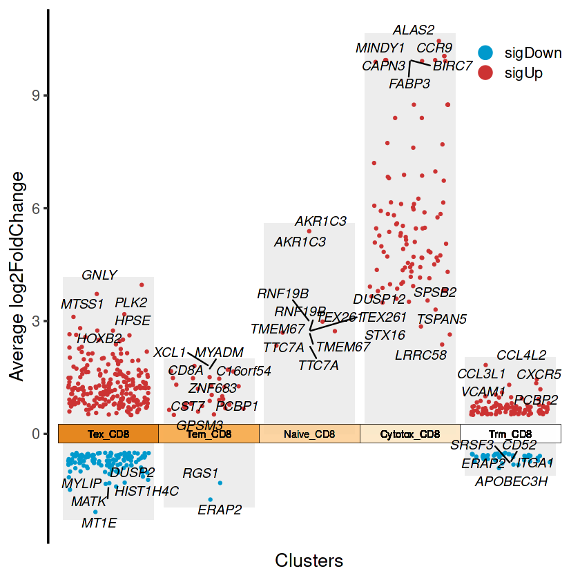
Cytotox_CD8   Naive_CD8     Tem_CD8     Tex_CD8     Trm_CD8 
        100           5          34         346         143 

jjVolcano(diffData = combined_results,
          tile.col = corrplot::COL2('PuOr', 15)[4:12],
          size  = 4,
          fontface = 'italic',
          base_size = 16,
          legend.position = c(0.9, 0.9),
          cluster.order = rev(unique(combined_results$cluster)))

2.富集分析

rm(list = ls())
setwd("/mnt/DEV_8T/zhaozm/seurat全流程/差异富集/")

##禁止转化为因子
options(stringsAsFactors = FALSE)

## 设置保存的目录
## 数据目录
data_dir <- "/mnt/DEV_8T/zhaozm/seurat全流程/差异富集/data"
if (!dir.exists(data_dir)) {
  dir.create(data_dir, recursive = TRUE)
}
## 图片目录
img_dir <- "/mnt/DEV_8T/zhaozm/seurat全流程/差异富集/img"

if (!dir.exists(img_dir)) {
  dir.create(img_dir, recursive = TRUE)
}

## 加载R包
library(readr)
library(msigdbr) 
library(gplots)
library(ggplot2)
library(clusterProfiler)
library(org.Hs.eg.db)
library(Seurat)
library(singleseqgset)
library(scRNAtoolVis)
library(dplyr)

载入程序包：‘gplots’

The following object is masked from ‘package:stats’:

    lowess

clusterProfiler v4.14.4 Learn more at https://yulab-smu.top/contribution-knowledge-mining/

Please cite:

Guangchuang Yu, Li-Gen Wang, Yanyan Han and Qing-Yu He.
clusterProfiler: an R package for comparing biological themes among
gene clusters. OMICS: A Journal of Integrative Biology. 2012,
16(5):284-287

载入程序包：‘clusterProfiler’

The following object is masked from ‘package:stats’:

    filter

载入需要的程序包：AnnotationDbi

载入需要的程序包：stats4

载入需要的程序包：BiocGenerics

载入程序包：‘BiocGenerics’

The following objects are masked from ‘package:stats’:

    IQR, mad, sd, var, xtabs

The following objects are masked from ‘package:base’:

    anyDuplicated, aperm, append, as.data.frame, basename, cbind,
    colnames, dirname, do.call, duplicated, eval, evalq, Filter, Find,
    get, grep, grepl, intersect, is.unsorted, lapply, Map, mapply,
    match, mget, order, paste, pmax, pmax.int, pmin, pmin.int,
    Position, rank, rbind, Reduce, rownames, sapply, saveRDS, setdiff,
    table, tapply, union, unique, unsplit, which.max, which.min

载入需要的程序包：Biobase

Welcome to Bioconductor

    Vignettes contain introductory material; view with
    'browseVignettes()'. To cite Bioconductor, see
    'citation("Biobase")', and for packages 'citation("pkgname")'.

载入需要的程序包：IRanges

载入需要的程序包：S4Vectors

载入程序包：‘S4Vectors’

The following object is masked from ‘package:clusterProfiler’:

    rename

The following object is masked from ‘package:gplots’:

    space

The following object is masked from ‘package:utils’:

    findMatches

The following objects are masked from ‘package:base’:

    expand.grid, I, unname

载入程序包：‘IRanges’

The following object is masked from ‘package:clusterProfiler’:

    slice

载入程序包：‘AnnotationDbi’

The following object is masked from ‘package:clusterProfiler’:

    select

载入需要的程序包：SeuratObject

载入需要的程序包：sp

载入程序包：‘sp’

The following object is masked from ‘package:IRanges’:

    %over%

载入程序包：‘SeuratObject’

The following object is masked from ‘package:IRanges’:

    intersect

The following object is masked from ‘package:S4Vectors’:

    intersect

The following object is masked from ‘package:BiocGenerics’:

    intersect

The following objects are masked from ‘package:base’:

    intersect, t

载入需要的程序包：Matrix

载入程序包：‘Matrix’

The following object is masked from ‘package:S4Vectors’:

    expand

载入需要的程序包：tidyverse

## 富集分析需要挂上代理
Sys.setenv("http_proxy"="http://10.16.46.126:7890")
Sys.setenv("https_proxy"="http://10.16.46.126:7890") 

## 读取差异分析之后的结果
tex_cd8_degs_fil <- read.csv(file = "./data/tex_cd8_差异基因.csv")
head(tex_cd8_degs_fil)

A data.frame: 6 × 7
	X	p_val	avg_log2FC	pct.1	pct.2	p_val_adj	gene
	<chr>	<dbl>	<dbl>	<dbl>	<dbl>	<dbl>	<chr>
1	GNLY	3.132400e-85	3.961162	0.543	0.147	6.199019e-81	GNLY
2	DUSP2	8.528781e-80	-1.330854	0.772	0.969	1.687846e-75	DUSP2
3	ENTPD1	2.926838e-58	2.506306	0.353	0.069	5.792213e-54	ENTPD1
4	KLRD1	6.800869e-58	2.146381	0.476	0.139	1.345892e-53	KLRD1
5	CALM1	5.550144e-57	-0.838229	0.868	0.975	1.098373e-52	CALM1
6	GAPDH	7.037207e-56	1.164210	0.969	0.978	1.392663e-51	GAPDH

ids_tex <- bitr(tex_cd8_degs_fil$gene, 'SYMBOL', 'ENTREZID', OrgDb = org.Hs.eg.db)
head(ids_tex)

'select()' returned 1:1 mapping between keys and columns

Warning message in bitr(tex_cd8_degs_fil$gene, "SYMBOL", "ENTREZID", OrgDb = org.Hs.eg.db):
“2.64% of input gene IDs are fail to map...”

A data.frame: 6 × 2
	SYMBOL	ENTREZID
	<chr>	<chr>
1	GNLY	10578
2	DUSP2	1844
3	ENTPD1	953
4	KLRD1	3824
5	CALM1	801
6	GAPDH	2597

tex_cd8_degs_fil <- merge(tex_cd8_degs_fil, ids_tex, by.x = 'gene', by.y = 'SYMBOL')
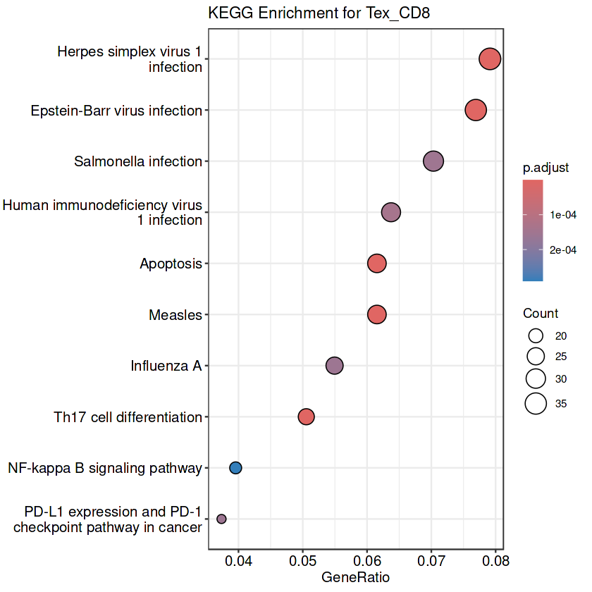
tex_cd8_kegg <- enrichKEGG(gene = tex_cd8_degs_fil$ENTREZID.x, organism = "hsa", pvalueCutoff = 1)
write.csv(as.data.frame(tex_cd8_kegg@result), file = "./data/tex_cd8_kegg_result.csv", row.names = FALSE)

dotplot(tex_cd8_kegg, showCategory = 10, title = "KEGG Enrichment for Tex_CD8")

## GSEA
library(clusterProfiler)
library(org.Hs.eg.db)
library(dplyr)
library(clusterProfiler)
library(enrichplot)
library(ggupset)
library(cowplot)

enrichplot v1.26.5 Learn more at https://yulab-smu.top/contribution-knowledge-mining/

Please cite:

Guangchuang Yu, Fei Li, Yide Qin, Xiaochen Bo, Yibo Wu and Shengqi
Wang. GOSemSim: an R package for measuring semantic similarity among GO
terms and gene products. Bioinformatics. 2010, 26(7):976-978

载入程序包：‘cowplot’

The following object is masked from ‘package:lubridate’:

    stamp

tex_cd8_degs_fil <- tex_cd8_degs_fil[order(tex_cd8_degs_fil$avg_log2FC, decreasing = TRUE),]
tex_markers_list <- setNames(as.numeric(tex_cd8_degs_fil$avg_log2FC), tex_cd8_degs_fil$ENTREZID.x)
tex_cd8_gsea_go <- gseGO(geneList = tex_markers_list, OrgDb = org.Hs.eg.db, ont = "ALL", pvalueCutoff = 0.05)
tex_cd8_gsea_go_arrange <- arrange(as.data.frame(tex_cd8_gsea_go@result), desc(abs(NES)))
write.csv(tex_cd8_gsea_go_arrange, file = "./data/tex_cd8_gsea_go_results.csv", row.names = FALSE)

using 'fgsea' for GSEA analysis, please cite Korotkevich et al (2019).


preparing geneSet collections...

GSEA analysis...

Warning message in fgseaMultilevel(pathways = pathways, stats = stats, minSize = minSize, :
“There were 2 pathways for which P-values were not calculated properly due to unbalanced (positive and negative) gene-level statistic values. For such pathways pval, padj, NES, log2err are set to NA. You can try to increase the value of the argument nPermSimple (for example set it nPermSimple = 10000)”
Warning message in fgseaMultilevel(pathways = pathways, stats = stats, minSize = minSize, :
“For some of the pathways the P-values were likely overestimated. For such pathways log2err is set to NA.”
leading edge analysis...

done...

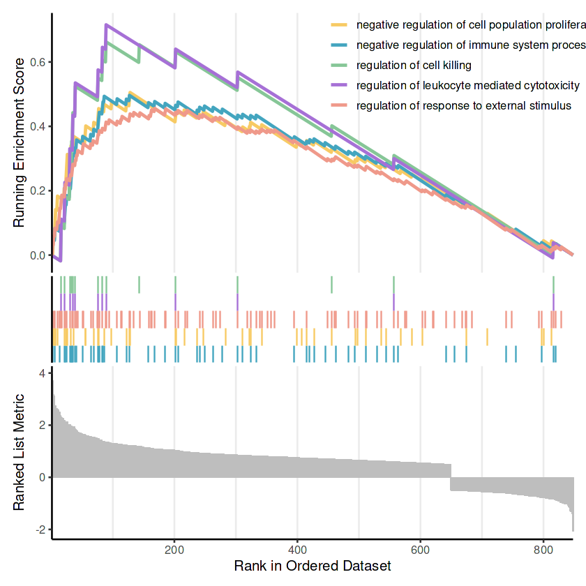
# 定义配色
color <- c("#f7ca64", "#43a5bf", "#86c697", "#a670d6", "#ef998a")

# 绘制 tex_cd8 的 GSEA-GO 图
## 上调
# 提取上调通路
upregulated_pathways <- tex_cd8_gsea_go@result %>%
  filter(NES > 0) %>%                       # 筛选上调通路
  arrange(desc(NES)) %>%                    # 按NES降序排列
  slice(1:5)                                # 选择前5条通路
# 绘制前5条上调通路的GSEA曲线
gsekp1_tex <- gseaplot2(
  tex_cd8_gsea_go,                          # GSEA结果对象
  geneSetID = upregulated_pathways$ID,      # 上调通路的ID向量
  pvalue_table = F,                      # 是否显示p值表
  base_size = 12,                           # 字体大小
  color = color # 可选颜色
)
upregulated_pathways$Description
# 显示图形
gsekp1_tex

negative regulation of immune system process
regulation of response to external stimulus
negative regulation of cell population proliferation
regulation of leukocyte mediated cytotoxicity
regulation of cell killing

Seurat单细胞处理流程之四：差异分析&富集分析

简介

1.差异分析

2.富集分析

Table of Contents