Seurat单细胞处理流程之九：拟时序分析

1 Apr 2025

rm(list = ls())
setwd("/mnt/DEV_8T/zhaozm/seurat全流程/monocle3/")

##禁止转化为因子
options(stringsAsFactors = FALSE)

## 设置保存的目录
## 数据目录
data_dir <- "/mnt/DEV_8T/zhaozm/seurat全流程/monocle3/data"
if (!dir.exists(data_dir)) {
  dir.create(data_dir, recursive = TRUE)
}
## 图片目录
img_dir <- "/mnt/DEV_8T/zhaozm/seurat全流程/monocle3/img"

if (!dir.exists(img_dir)) {
  dir.create(img_dir, recursive = TRUE)
}

library(celldex)
library(assertthat)
library(monocle)
library(monocle3)
library(Seurat)
library(tidyverse)
library(Matrix)
library(stringr)
library(dplyr)
library(tricycle)
library(scattermore)
library(scater)
library(patchwork)
library(CCA)
library(clustree)
library(cowplot)
library(SCpubr)
library(UCell)
library(irGSEA)
library(GSVA)
library(GSEABase)
library(harmony)
library(plyr)
library(randomcoloR)
library(CellChat)
library(future)
library(ggforce)
library(ggsci)

set.seed(12345)
## 并将seurat对象转换为CDS对象
sce <- read_rds(file = "../差异富集/data/CD4注释后.rds")
## 提取相应的细胞
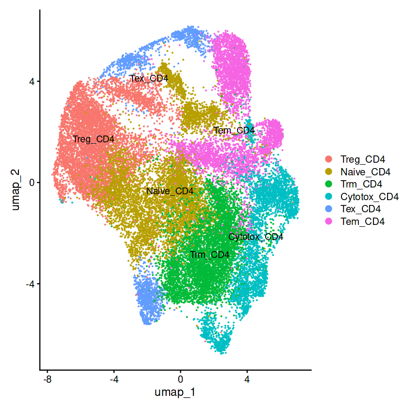
DimPlot(sce,label = T)
unique(sce$celltype)
seu_obj = subset(sce,idents=c("Treg_CD4","Naive_CD4","Tex_CD4"))

<ol class=list-inline><li>‘Treg_CD4’</li><li>‘Naive_CD4’</li><li>‘Trm_CD4’</li><li>‘Cytotox_CD4’</li><li>‘Tex_CD4’</li><li>‘Tem_CD4’</li></ol>

# 提取seu_obj对象中RNA数据的原始计数矩阵
data <- GetAssayData(seu_obj, assay = 'RNA', slot = 'counts')  

# 提取seu_obj对象中的细胞元数据
cell_metadata <- seu_obj@meta.data 

# 创建基因注释数据框，基因名为data行名
gene_annotation <- data.frame(gene_short_name = rownames(data)) 

# 设置gene_annotation的行名为基因名
rownames(gene_annotation) <- rownames(data) 

# 和monocle2一样，构建CellDataSet (cds) 对象，输入包括表达矩阵、细胞元数据、基因注释
cds <- new_cell_data_set(data,
                         cell_metadata = cell_metadata,
                         gene_metadata = gene_annotation)  
                         
# 对cds进行预处理，默认使用PCA降维，保留50个主成分                       
cds <- preprocess_cds(cds, num_dim = 50)  
# cds<-align_cds(cds,alignment_group="orig.ident")#去除批次(可选)

 # 使用PCA方法进行降维
cds <- reduce_dimension(cds, preprocess_method = "PCA") 

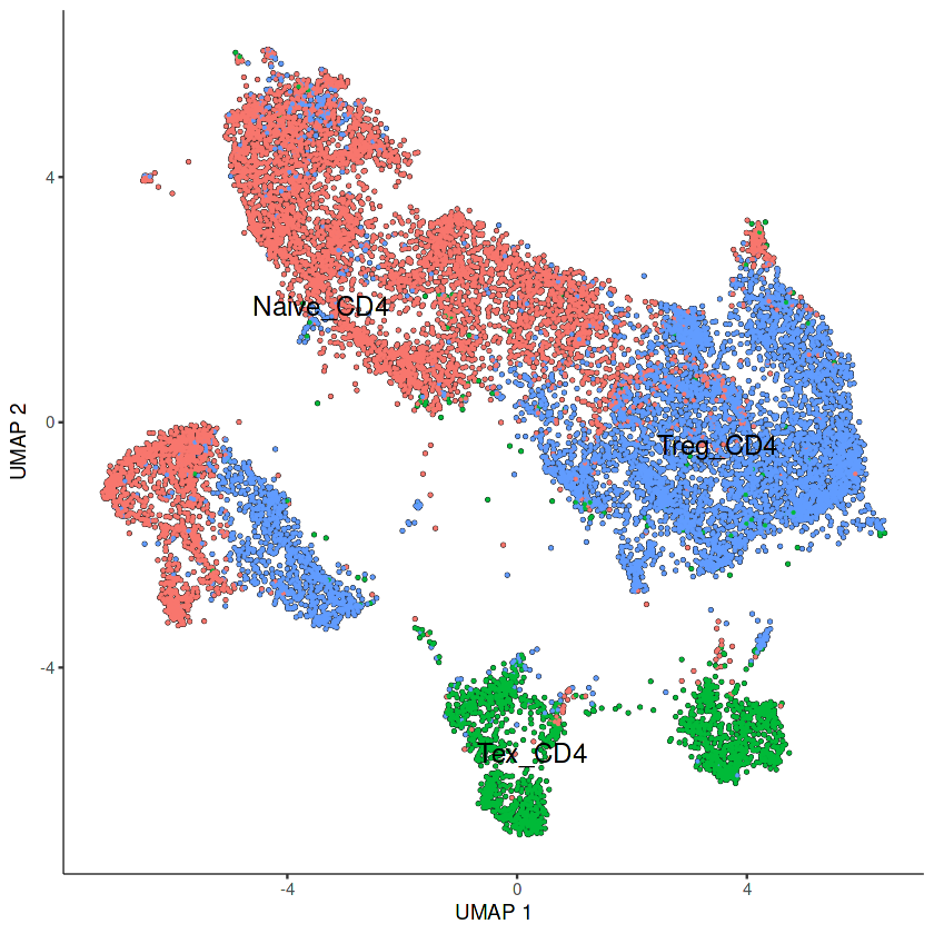
# 展示monocle3聚类的细胞类型
p1=plot_cells(cds, color_cells_by="celltype",cell_size=0.5,group_label_size=5)
p1

No trajectory to plot. Has learn_graph() been called yet?

#将monocle3对象与我们的seurat的UMAP降维相结合
# 提取Monocle3中已计算的UMAP降维坐标
cds.embed <- cds@int_colData$reducedDims$UMAP  

# 提取Seurat对象中计算的UMAP坐标
int.embed <- Embeddings(seu_obj, reduction = "umap")  

# 将Seurat和Monocle3的细胞顺序对齐
int.embed <- int.embed[rownames(cds.embed),]  

 # 将Seurat的UMAP坐标赋值给Monocle3的UMAP坐标
cds@int_colData$reducedDims$UMAP <- int.embed 

# 使用Louvain算法在UMAP空间进行细胞聚类
# cluster聚类
cds <- cluster_cells(cds, reduction_method = "UMAP", cluster_method = 'louvain')  

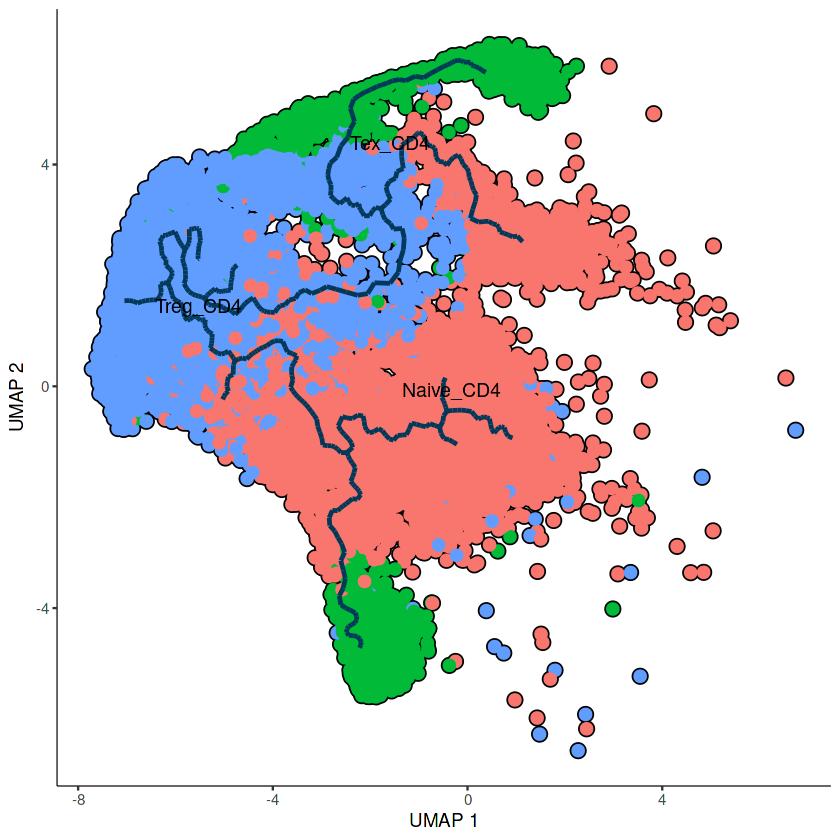
#轨迹推断
mycds1 <- learn_graph(cds,
                      verbose=T,
                      use_partition=T,## 根据细胞数量选择
                      learn_graph_control=list(minimal_branch_len=35,#在图修剪过程中要保留的分支直径路径的最小长度。默认值是10。
                                               euclidean_distance_ratio=0.1#生成树中两个末端节点的欧氏距离与生成树上允许连接的任何连接点之间的最大距离之比。默认值为1。
                      ))

## 画图展示
plot_cells(mycds1, 
           color_cells_by = 'celltype',
           label_groups_by_cluster=FALSE,
           label_leaves=FALSE,
           label_branch_points=FALSE,
           cell_size=2,group_label_size=4,
           trajectory_graph_color='#023858',
           trajectory_graph_segment_size = 1)

#定义root cell, 推断拟时方向
## 根据shiney里的选择
## 选择起点
# mycds1 <- order_cells(mycds1)
# jupyter内不支持shiny，此处建议在Rstudio内做

#在monocle3分析中，我们使用graph_test函数分析过拟时差异基因，这个过程比较慢
library(ClusterGVis)
library(monocle3)
library(dplyr)

# modulated_genes <- graph_test(mycds1, neighbor_graph = "principal_graph", cores = 8)
# ## 保存差异基因
# write.csv(modulated_genes,file = "./data/cd4_modulated_genes.csv",row.names = T)

## 使用clusterGvis包进行绘制图片
#读取分析的文件
load(file = './data/cd4_Monocle3_cds_peu.RData')
## 读取差异基因
modulated_genes <- read.csv(file = "./data/cd4_modulated_genes.csv",row.names = 1)
genes <- row.names(subset(modulated_genes, q_value == 0 ))
mat <- pre_pseudotime_matrix(cds_obj = mycds1,
                             gene_list = genes)

# check
head(mat[1:5,1:5])

A matrix: 5 × 5 of type dbl
	1	2	3	4	5
ISG15	-1.767955	-1.767522	-1.767089	-1.766656	-1.766223
TNFRSF18	-2.168919	-2.168531	-2.168143	-2.167755	-2.167367
TNFRSF4	-2.118236	-2.117874	-2.117511	-2.117149	-2.116786
RPL22	2.519977	2.519398	2.518820	2.518242	2.517663
TNFRSF9	-2.220663	-2.220247	-2.219831	-2.219415	-2.218999

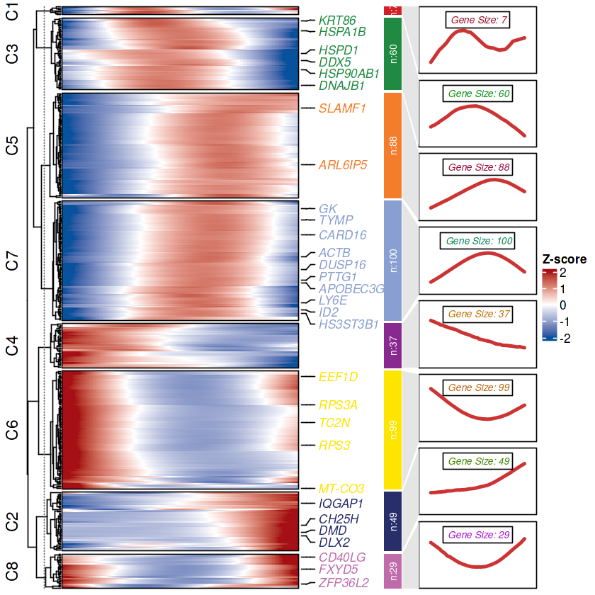
# kmeans
ck <- clusterData(exp = mat,
                  cluster.method = "kmeans",
                  cluster.num = 8)

## 热图
visCluster(object = ck,
           plot.type = "both",
           add.sampleanno = F,
           markGenes = sample(rownames(mat),30,replace = F))

0 genes excluded.

This palatte have 20 colors!

Seurat单细胞处理流程之九：拟时序分析

Table of Contents