Seurat单细胞处理流程之八：pySCENIC转录因子分析-R可视化

rm(list = ls())
setwd("/mnt/DEV_8T/zhaozm/seurat全流程/pyscenic/")

##禁止转化为因子
options(stringsAsFactors = FALSE)

## 设置保存的目录
## 数据目录
data_dir <- "/mnt/DEV_8T/zhaozm/seurat全流程/pyscenic/data"
if (!dir.exists(data_dir)) {
  dir.create(data_dir, recursive = TRUE)
}
## 图片目录
img_dir <- "/mnt/DEV_8T/zhaozm/seurat全流程/pyscenic/img"

if (!dir.exists(img_dir)) {
  dir.create(img_dir, recursive = TRUE)
}

options(repr.plot.width = 16, repr.plot.height = 10)
## 设置jupyter画板的全局参数

##可视化
library(Seurat)
library(SCopeLoomR)
library(AUCell)
library(SCENIC)
library(dplyr)
library(KernSmooth)
library(RColorBrewer)
library(plotly)
library(BiocParallel)
library(grid)
library(ComplexHeatmap)
library(data.table)
library(scRNAseq)
library(patchwork)
library(ggplot2) 
library(stringr)
library(circlize)

## 读取上一步的loom文件
loom <- open_loom('./out_pbmc_SCENIC.loom') 
regulons_incidMat <- get_regulons(loom, column.attr.name="Regulons")

regulons_incidMat[1:4,1:4] 

A matrix: 4 × 4 of type int

	AL627309.1	AP006222.2	RP11-206L10.2	RP11-206L10.9
AHR(+)	0	0	0	0
APEX1(+)	0	0	0	0
ARID3A(+)	0	0	0	0
ARNTL(+)	0	0	0	0

regulons <- regulonsToGeneLists(regulons_incidMat)
regulonAUC <- get_regulons_AUC(loom,column.attr.name='RegulonsAUC')
regulonAucThresholds <- get_regulon_thresholds(loom)


tail(regulonAucThresholds[order(as.numeric(names(regulonAucThresholds)))])

<dl class=dl-inline><dt>0.287117464540207</dt><dd>‘JUN(+)’</dd><dt>0.288565330122853</dt><dd>‘FOXP1(+)’</dd><dt>0.293575067056502</dt><dd>‘TAF7(+)’</dd><dt>0.312024320517666</dt><dd>‘KLF2(+)’</dd><dt>0.37288804895773</dt><dd>‘XBP1(+)’</dd><dt>0.440506596181331</dt><dd>‘HMGB1(+)’</dd></dl>

embeddings <- get_embeddings(loom)  
close_loom(loom)
rownames(regulonAUC)
# names(regulons)

#### 2.导入seurat对象和加载的regulon信息进行匹配应对
sce <- readRDS(file = "../降维注释/data/pbmc注释后.rds")
# 取交集
sub_regulonAUC <- regulonAUC[,match(colnames(sce),colnames(regulonAUC))]
dim(sub_regulonAUC)

<ol class=list-inline><li>272</li><li>2638</li></ol>

sce 

An object of class Seurat 
13714 features across 2638 samples within 1 assay 
Active assay: RNA (13714 features, 2000 variable features)
 3 layers present: counts, data, scale.data
 2 dimensional reductions calculated: pca, umap

#确认是否一致
identical(colnames(sub_regulonAUC), colnames(sce))

TRUE

# 构建细胞类型注释信息
cellTypes <- data.frame(row.names = colnames(sce), 
                        celltype = sce$celltype)
head(cellTypes)
sub_regulonAUC[1:4,1:4] 

A data.frame: 6 × 1

	celltype
	<chr>
AAACATACAACCAC-1	Memory CD4 T
AAACATTGAGCTAC-1	B
AAACATTGATCAGC-1	Memory CD4 T
AAACCGTGCTTCCG-1	CD14+ Mono
AAACCGTGTATGCG-1	NK
AAACGCACTGGTAC-1	Memory CD4 T

AUC for 4 regulons (rows) and 4 cells (columns).

Top-left corner of the AUC matrix:
           cells
regulons    AAACATACAACCAC-1 AAACATTGAGCTAC-1 AAACATTGATCAGC-1 AAACCGTGCTTCCG-1
  AHR(+)          0.00000000      0.000000000      0.032069971      0.040233236
  APEX1(+)        0.14577259      0.232264334      0.072886297      0.187074830
  ARID3A(+)       0.01093294      0.000000000      0.002935698      0.096007451
  ARNTL(+)        0.02461937      0.005250513      0.013578447      0.002996437

table(sce$celltype)
# 根据自己需要的信息进行划分
selectedResolution <- "celltype"
cellsPerGroup <- split(rownames(cellTypes),cellTypes[,selectedResolution]) 
# 保留唯一/非重复的 regulon
sub_regulonAUC <- sub_regulonAUC[onlyNonDuplicatedExtended(rownames(sub_regulonAUC)),] 
dim(sub_regulonAUC)

           B   CD14+ Mono        CD8 T           DC FCGR3A+ Mono Memory CD4 T 
         344          483          281           30          161          459 
 Naive CD4 T           NK     Platelet 
         721          145           14 

272 2638

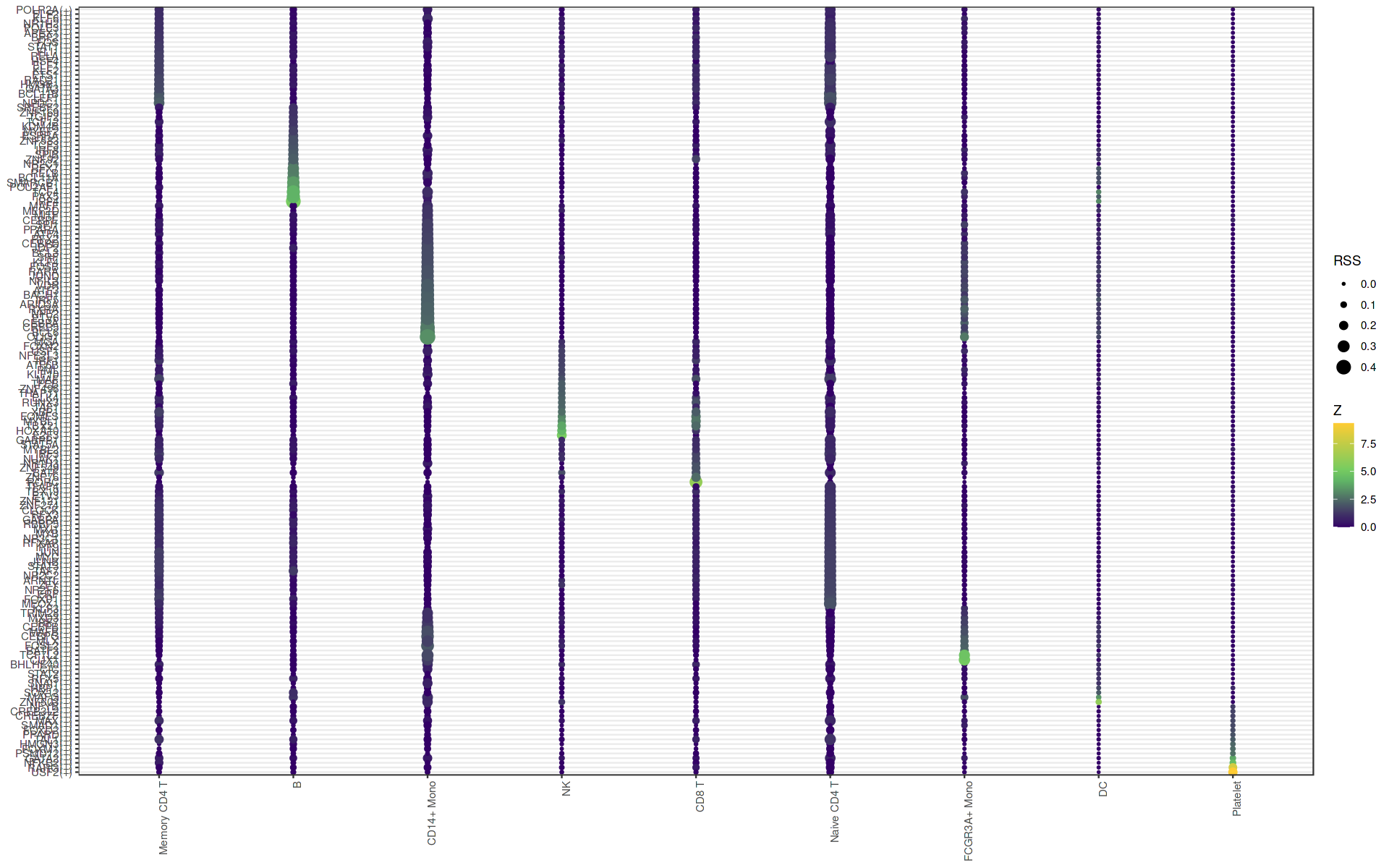
## 计算regulon特异性分数(RSS)
# regulon特异性分数(Regulon Specificity Score, RSS)
selectedResolution <- "celltype"
rss <- calcRSS(AUC=getAUC(sub_regulonAUC), 
               cellAnnotation=cellTypes[colnames(sub_regulonAUC),selectedResolution]) 
rss=na.omit(rss) 
rssPlot <- plotRSS(rss,
                   labelsToDiscard = NULL, # 指定需要在热图中排除的行或列标签
                   zThreshold = 1, # 设定调控子的阈值，默认1
                   cluster_columns = FALSE, # 是否对列进行聚类
                   order_rows = T, # 是否对行进行排序
                   thr = 0.01, # 阈值参数，用于过滤 RSS 值。默认0.01
                   varName = "cellType",
                   col.low = '#330066',  
                   col.mid = '#66CC66',  
                   col.high= '#FFCC33',
                   revCol = F,
                   verbose = TRUE
)
rssPlot
options(bitmapType = "cairo")

p <- plotly::ggplotly(rssPlot$plot)
p <- p %>%
  layout(
    title = "RSS Plot",
    xaxis = list(title = "Celltypes"),
    yaxis = list(title = "Regulons")
  )


p

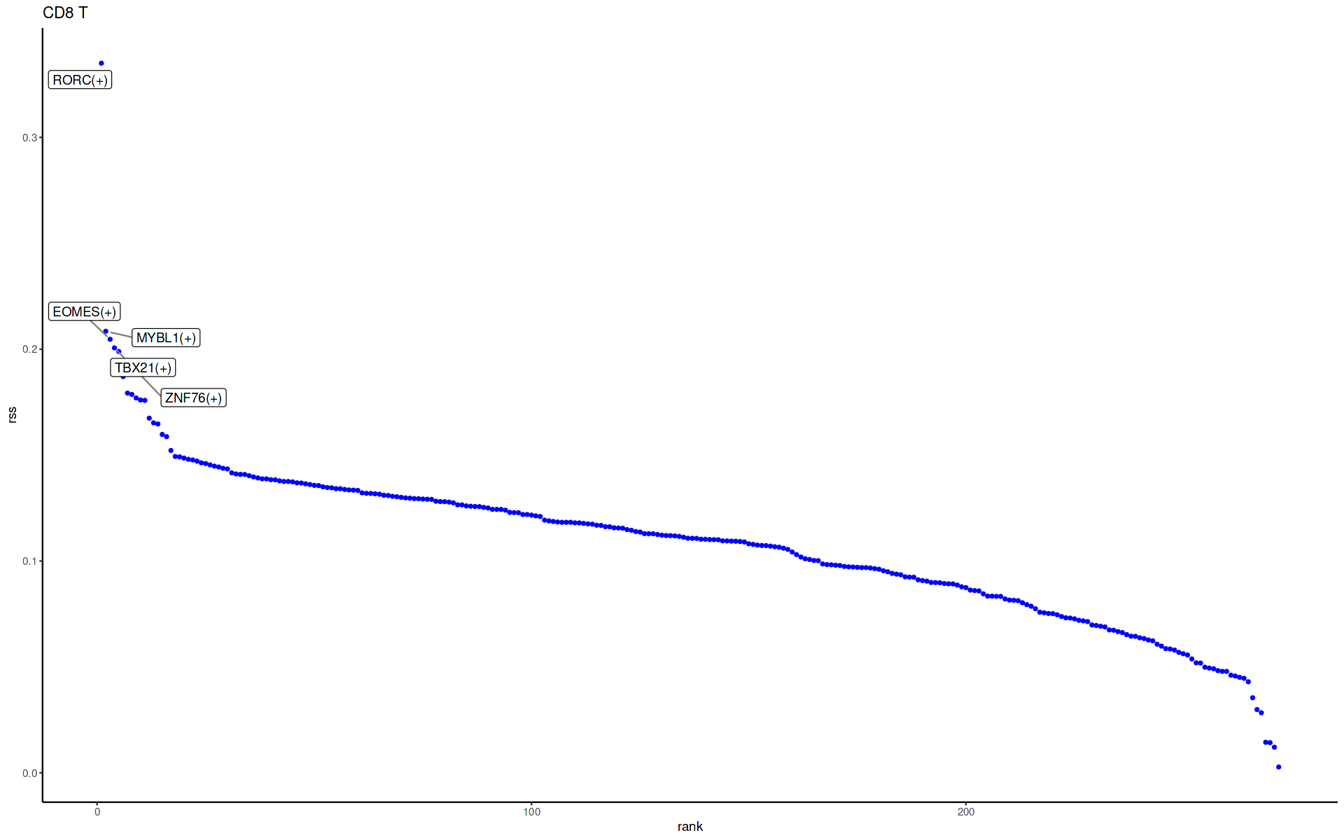
plotRSS_oneSet(rss, setName = "CD8 T") # cluster ID

# 计算每个细胞组中各调控子(regulon)的平均活性，并将这些平均活性值存储在一个矩阵中
# cellsPerGroup这里得到是不同细胞群中的样本列表
# function(x)rowMeans(getAUC(sub_regulonAUC)[,x])可以计算每个细胞群的regulon平均AUC值
regulonActivity_byGroup <- sapply(cellsPerGroup,
                                  function(x) 
                                    rowMeans(getAUC(sub_regulonAUC)[,x]))
range(regulonActivity_byGroup)

0.406250519055341

# 对结果进行归一化
regulonActivity_byGroup_Scaled <- t(scale(t(regulonActivity_byGroup),
                                          center = T, scale=T)) 

# 同一个regulon在不同cluster的scale处理
dim(regulonActivity_byGroup_Scaled)
regulonActivity_byGroup_Scaled=regulonActivity_byGroup_Scaled[]
regulonActivity_byGroup_Scaled=na.omit(regulonActivity_byGroup_Scaled)

272

library(dplyr) 
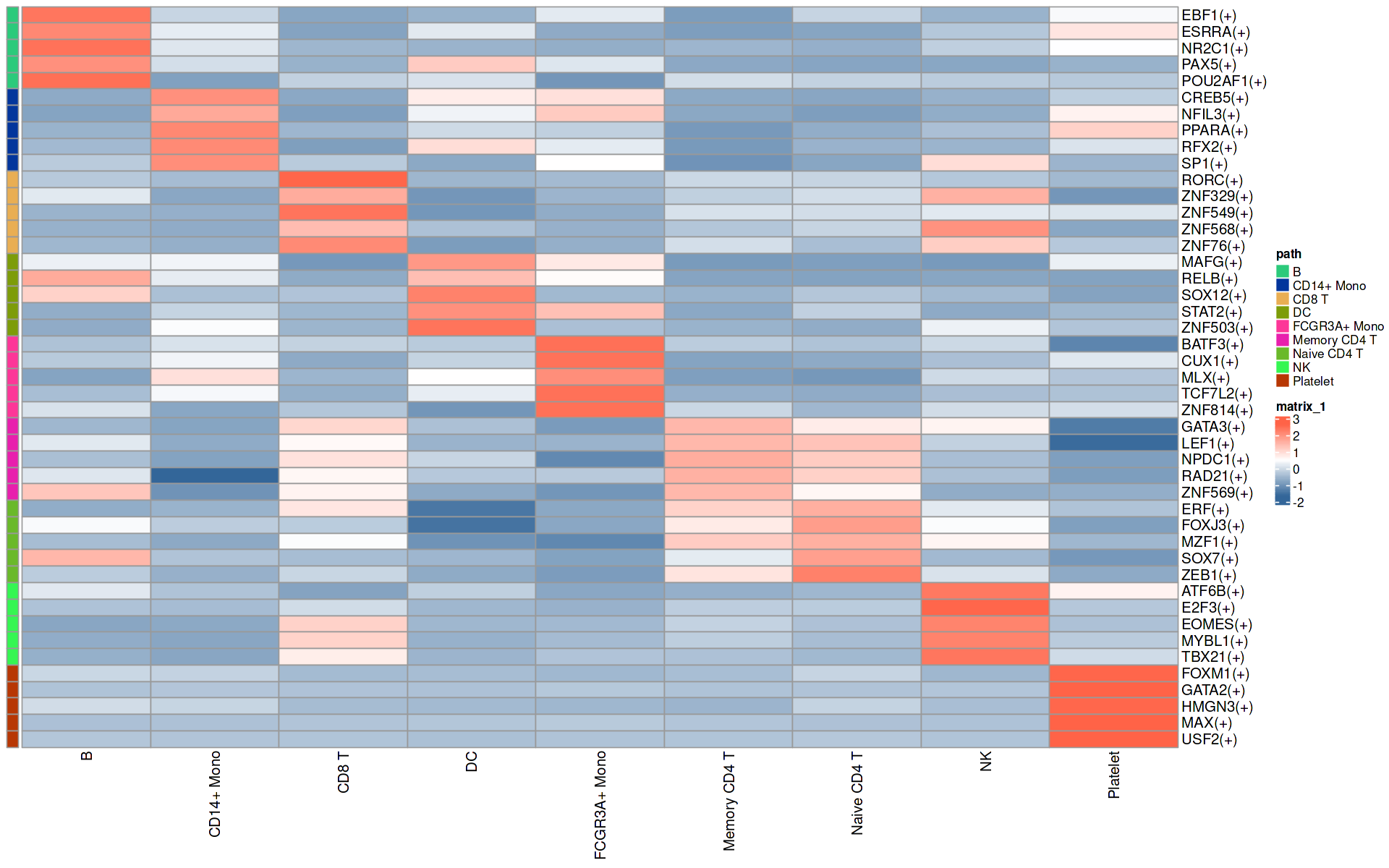
rss=regulonActivity_byGroup_Scaled
head(rss)
df = do.call(rbind,
             lapply(1:ncol(rss), function(i){
               dat= data.frame(
                 path  = rownames(rss), # 当前regulon的名称
                 cluster = colnames(rss)[i], # 当前cluster的名称
                 sd.1 = rss[,i], # 当前cluster中每个调控因子的值
                 sd.2 = apply(rss[,-i], 1, median)  #除了当前cluster之外的所有cluster 中该调控因子的中位值
               )
             }))
df$fc = df$sd.1 - df$sd.2

top5 <- df %>% 
  group_by(cluster) %>% 
  top_n(5, fc)
rowcn = data.frame(path = top5$cluster) 
n = rss[top5$path,] 

breaksList = seq(-1.5, 1.5, by = 0.1)
colors <- colorRampPalette(c("#336699", "white", "tomato"))(length(breaksList))

A matrix: 6 × 9 of type dbl

	B	CD14+ Mono	CD8 T	DC	FCGR3A+ Mono	Memory CD4 T	Naive CD4 T	NK	Platelet
AHR(+)	-0.01079404	0.04430424	-0.2551160	-1.9998138	-0.2291863	0.3974552	-0.2097201	0.3835017	1.8793691
APEX1(+)	0.59661847	-0.27602042	-0.3590493	1.4097815	0.4591368	0.6754387	0.4772521	-1.2602244	-1.7229334
ARID3A(+)	-0.66501429	1.40575469	-0.8497800	0.7304750	0.7690242	-0.7559845	-0.8801283	-0.9630327	1.2086858
ARNTL(+)	-0.36067150	-0.77655701	0.5700973	-1.2267423	-1.4662731	0.3939737	0.8414152	1.4448105	0.5799473
ATF1(+)	0.08143190	-0.18468715	0.6530174	-1.1488711	0.8302434	0.5776227	0.4197098	0.8450898	-2.0735568
ATF3(+)	-0.67963155	1.50856719	-0.7699783	0.9926624	1.3901314	-0.7276563	-0.8960423	-0.6147384	-0.2033142

pheatmap(n,
         annotation_row = rowcn,
         color = colors,
         cluster_rows = F,
         cluster_cols = FALSE,
         show_rownames = T,
         #gaps_col = cumsum(table(annCol$Type)),  # 使用排序后的列分割点
         #gaps_row = cumsum(table(annRow$Methods)), # 行分割
         fontsize_row = 12,
         fontsize_col = 12,
         annotation_names_row = FALSE)

#  特定转录因子绘图
library(SummarizedExperiment)
seurat.data <- sce
Idents(seurat.data) <- "celltype"
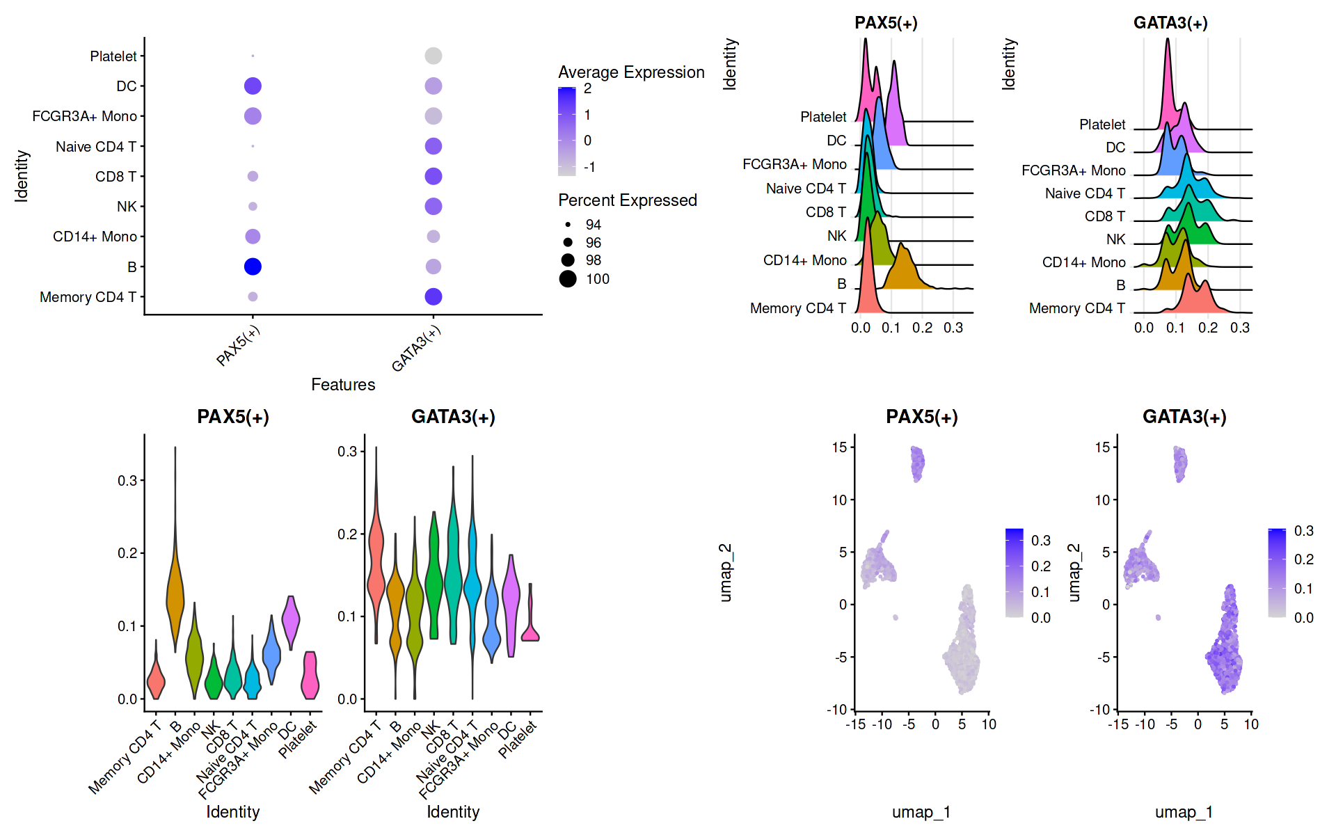
regulonsToPlot = c("PAX5(+)","GATA3(+)")
regulonsToPlot %in% row.names(sub_regulonAUC)
seurat.data@meta.data = cbind(seurat.data@meta.data ,
                              t(assay(sub_regulonAUC[regulonsToPlot,])))

# Vis
p1 = DotPlot(seurat.data, features = unique(regulonsToPlot)) + RotatedAxis()
p2 = RidgePlot(seurat.data, features = regulonsToPlot , ncol = 2) 
p3 = VlnPlot(seurat.data, features = regulonsToPlot,pt.size = 0)
p4 = FeaturePlot(seurat.data,features = regulonsToPlot)

wrap_plots(p1, p2, p3, p4, ncol = 2, widths = c(5, 5), heights = c(5, 5))

<ol class=list-inline><li>TRUE</li><li>TRUE</li></ol>

Picking joint bandwidth of 0.00626

Picking joint bandwidth of 0.0105

• 心得
• 学习
• seurat
• 单细胞流程
• python